The other day I was playing around with some Bureau of Meteorology data for my little patch of the Adelaide Hills (free data — how can I resist?), when I discovered an interesting trend.
Living on a little farm with a small vineyard, I’m rather keen on understanding our local weather trends. Being a scientist, I’m also rather inclined to analyse data.
My first question was given the strong warming trend here and everywhere else, plus ample evidence of changing rainfall patterns in Australia (e.g., see here, here, here, here, here), was it drying out, getting wetter, or was the seasonal pattern of rainfall in my area changing?
I first looked to see if there was any long-term trend in total annual rainfall over time. Luckily, the station records nearest my farm go all the way back to 1890:
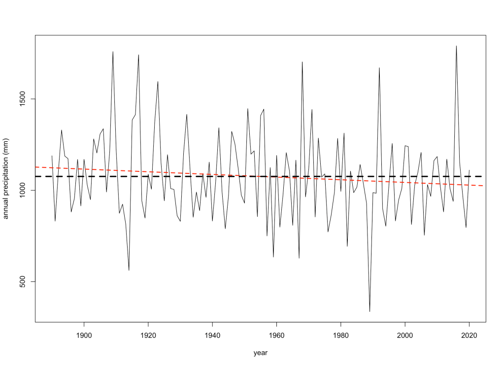
While the red line might suggest a slight decrease since the late 19th Century, it’s no different to an intercept-only model (evidence ratio = 0.84) — no trend.
Here’s the R code to do that analysis (you can download the data here, or provide your own data in the same format):
## IMPORT MONTHLY PRECIPITATION DATA
dat <- read.table("monthlyprecipdata.csv", header=T, sep=",")

## CALCULATE ANNUAL VECTORS
precip.yr.sum <- xtabs(dat$Monthly.Precipitation.Total..millimetres. ~ dat$Year)
precip.yr.sum <- precip.yr.sum[-length(precip.yr.sum)]
year.vec <- as.numeric(names(precip.yr.sum))

## PLOT
plot(year.vec, as.numeric(precip.yr.sum), type="l", pch=19, xlab="year", ylab="annual precipitation (mm)")
fit.yr <- lm(precip.yr.sum ~ year.vec)
abline(fit.yr, lty=2, lwd=2, col="red")
abline(h=mean(as.numeric(precip.yr.sum)),lty=2, lwd=3)

## TEST FOR TREND
# functions
AICc <- function(...) {
  models <- list(...)
  num.mod <- length(models)
  AICcs <- numeric(num.mod)
  ns <- numeric(num.mod)
  ks <- numeric(num.mod)
  AICc.vec <- rep(0,num.mod)
  for (i in 1:num.mod) {
    if (length(models[[i]]$df.residual) == 0) n <- models[[i]]$dims$N else n <- length(models[[i]]$residuals)
    if (length(models[[i]]$df.residual) == 0) k <- sum(models[[i]]$dims$ncol) else k <- (length(models[[i]]$coeff))+1
    AICcs[i] <- (-2*logLik(models[[i]])) + ((2*k*n)/(n-k-1))
    ns[i] <- n
    ks[i] <- k
    AICc.vec[i] <- AICcs[i]
  }
  return(AICc.vec)
}

delta.AIC <- function(x) x - min(x) ## where x is a vector of AIC
weight.AIC <- function(x) (exp(-0.5*x))/sum(exp(-0.5*x)) ## Where x is a vector of dAIC
ch.dev <- function(x) ((( as.numeric(x$null.deviance) - as.numeric(x$deviance) )/ as.numeric(x$null.deviance))*100) ## % change in deviance, where x is glm object

linreg.ER <- function(x,y) { # where x and y are vectors of the same length; calls AICc, delta.AIC, weight.AIC functions
  fit.full <- lm(y ~ x); fit.null <- lm(y ~ 1)
  AIC.vec <- c(AICc(fit.full),AICc(fit.null))
  dAIC.vec <- delta.AIC(AIC.vec); wAIC.vec <- weight.AIC(dAIC.vec)
  ER <- wAIC.vec[1]/wAIC.vec[2]
  r.sq.adj <- as.numeric(summary(fit.full)[9])
  return(c(ER,r.sq.adj))
}

linreg.ER(year.vec, as.numeric(precip.yr.sum))


