Want a permanent DOI assigned to your data and code? Follow this simple recipe

2 11 2021

These days with data and code often required to be designated as open-source, licenced, and fully trackable for most manuscript submissions to a peer-reviewed journal, it’s easy to get lost in the multitude of platforms and options available. In most cases, we no longer have much of a choice to do so, even if you are reticent (although the benefits of posting your data and code online immediately far outweigh any potential disadvantages).

But do you post your data and code on the Open Science Framework (free), Github (free), Figshare (free), Zenodo (free, but donations encouraged), Dryad ($), or Harvard Dataverse (free) (and so on, and so on, …)? Pick your favourite. Another issue that arises is that even if you have solved the first dilemma, how do you obtain a digital object identifier (DOI) for your data and/or code?

Again, there are many ways to do this, and some methods are more automated than other. That said, I do have a preference that is rather easy to implement that I’d thought I’d share with you here.

The first requirement is getting yourself a (free) Github account. What’s Github? Github is one of the world’s largest communities of developers, where code for all manner of types and uses can be developed, shared, updated, collaborated, shipped, and maintained. It might seem a bit overwhelming for non-developers, but if you strip it down to its basics, it’s straightforward to use as a simple repository for your code and data. Of course, Github is designed for so much more than just this (software development collaboration being one of the main ones), but you don’t need to worry about that for now.

Step 1

Once you create an account, you can start creating ‘repositories’, which are essentially just sections of your account dedicated to specific code (and data). I mostly code in R, so I upload my R code text files and associated datasets to these repositories, and spend a good deal of effort on making the Readme.md file highly explanatory and easy to follow. You can check out some of mine here.

Ok. So, you have a repository with some code and data, you’ve explained what’s going on and how the code works in the Readme file, and now you want a permanent DOI that will point to the repository (and any updates) for all time.

Github doesn’t do this by itself, but it integrates seamlessly with another platform — Zenodo — that does. Oh no! Not another platform! Yes, I’m afraid so, but it’s not as painful as you might expect.

Read the rest of this entry »


The ε-index app: a fairer way to rank researchers with citation data

9 11 2020

Back in April I blogged about an idea I had to provide a more discipline-, gender-, and career stage-balanced way of ranking researchers using citation data.

Most of you are of course aware of the ubiquitous h-index, and its experience-corrected variant, the m-quotient (h-index ÷ years publishing), but I expect that you haven’t heard of the battery of other citation-based indices on offer that attempt to correct various flaws in the h-index. While many of them are major improvements, almost no one uses them.

Why aren’t they used? Most likely because they aren’t easy to calculate, or require trawling through both open-access and/or subscription-based databases to get the information necessary to calculate them.

Hence, the h-index still rules, despite its many flaws, like under-emphasising a researcher’s entire body of work, gender biases, and weighting towards people who have been at it longer. The h-index is also provided free of charge by Google Scholar, so it’s the easiest metric to default to.

So, how does one correct for at least some of these biases while still being able to calculate an index quickly? I think we have the answer.

Since that blog post back in April, a team of seven scientists and I from eight different science disciplines (archaeology, chemistry, ecology, evolution & development, geology, microbiology, ophthalmology, and palaeontology) refined the technique I reported back then, and have submitted a paper describing how what we call the ‘ε-index’ (epsilon index) performs.

Read the rest of this entry »


Dangers of forcing regressions through the origin

17 10 2017

correlationsI had an interesting ‘discussion’ on Twitter yesterday that convinced me the topic would make a useful post. The specific example has nothing whatsoever to do with conservation, but it serves as a valuable statistical lesson for all concerned about demonstrating adequate evidence before jumping to conclusions.

The data in question were used in a correlation between national gun ownership (guns per capita) and gun-related deaths and injuries (total deaths and injuries from guns per 100,000 people) (the third figure in the article). As you might intuitively expect, the author concluded that there was a positive correlation between gun-related deaths and injuries, and gun ownership:

image-20160307-30436-2rzo6k

__

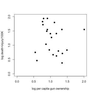
Now, if you’re an empirical skeptic like me, there was something fishy about that fitted trend line. So, I replotted the data (available here) using Plot Digitizer (if you haven’t yet discovered this wonderful tool for lifting data out of figures, you would be wise to get it now), and ran a little analysis of my own in R:

Rplot01

Just doing a little 2-parameter linear model (y ~ α + βx) in R on these log-log data (which means, it’s assumed to be a power relationship), shows that there’s no relationship at all — the intercept is 1.3565 (± 0.3814) in log space (i.e., 101.3565 = 22.72), and there’s no evidence for a non-zero slope (in fact, the estimated slope is negative at -0.1411, but it has no support). See R code here.

Now, the author pointed out what appears to be a rather intuitive requirement for this analysis — you should not have a positive number of gun-related deaths/injuries if there are no guns in the population; in other words, the relationship should be forced to go through the origin (xy = 0, 0). You can easily do this in R by using the lm function and setting the relationship to y ~ 0 + x; see code here). Read the rest of this entry »


%d bloggers like this: