Imagine growing up beside the eastern Mediterranean Sea 14,000 years ago. You’re an accomplished sailor of the small watercraft you and your fellow villagers make, and you live off both the sea and the land.
But times have been difficult — there just isn’t the same amount of game or fish around as when you were a child. Maybe it’s time to look elsewhere for food.
Now imagine going farther than ever before in your little boat, accompanied maybe by a few others, when suddenly you spot something on the horizon. Is that an island?
The western coast of Cyprus. CJA Bradshaw / Flinders University
When you beach your boat to have a look around, you can’t believe what you’re seeing — tiny boar-sized hippos and horse-sized elephants that look like babies to your eyes. There are so many of them, and you’re hungry after the long journey.
The diminutive beasts don’t seem to show any fear. You easily kill a few and preserve the meat as best you can for the long journey back.
When you get home, you are excited to let everyone in the village know what you’ve found. Soon enough, you organise a major expedition back to the island.
Of course, we’ll never know if this kind of scenario took place, but it’s a plausible story of how and when the first humans managed to get to Cyprus. It also illustrates how they might have quickly brought about the demise of the tiny hippopotamusPhanourios minor, as well as the dwarf elephantPalaeoloxodon cypriotes.
If several fossils of an extinct population or species are dated, we can estimate how long ago the extinction event took place. In our new paper, we describe CRIWM, a new method to estimate extinction time using times series of fossils whose ages have been measured by radiocarbon dating.And yes, there’s an R package — Rextinct — to go with that!
While the Earth seems to gather all the conditions for life to thrive, over 99.9% of all species that ever lived are extinct today. From a distance, pristine landscapes might look similar today and millennia ago: blue seas with rocky and sandy coasts and grasslands and mountain ranges watered by rivers and lakes and covered in grass, bush and trees.
But zooming in, the picture is quite different because species identities have never stopped changing — with ‘old’ species being slowly replaced by ‘new’ ones. Fortunately, much like the collection of books in the library summarises the history of literature, the fossilised remnants of extinct organisms represent an archive of the kinds of creatures that have ever lived. This fossil record can be used to determine when and why species disappear. In that context, measuring the age of fossils is a useful task for studying the history of biodiversity and its connections to the planet’s present.
In our new paper published in the journal Quaternary Geochronology (1), we describe CRIWM (calibration-resampled inverse-weighted McInerny), a statistical method to estimate extinction time using times series of fossils that have been dated using radiocarbon dating.
Why radiocarbon dating? Easy. It is the most accurate and precise chronometric method to date fossils younger than 50,000 to 55,000 years old (2, 3). This period covers the Holocene (last 11,700 years or so), and the last stretch of the late Pleistocene (~ 130,000 years ago to the Holocene), a crucial window of time witnessing the demise of Quaternary megafauna at a planetary scale (4) (see videos here, here and here), and the global spread of anatomically modern humans (us) ‘out of Africa’ (see here and here).
Why do we need a statistical method? Fossilisation (the process of body remains being preserved in the rock record) is rare and finding a fossil is so improbable that we need maths to control for the incompleteness of the fossil record and how this fossil record relates to the period of survival of an extinct species.
A brief introduction to radiocarbon dating
First, let’s revise the basics of radiocarbon dating (also explained here and here). This chronometric technique measures the age of carbon-rich organic materials — from shells and bones to the plant and animal components used to write an ancient Koran, make a wine vintage and paint La Mona Lisa and Neanderthal caves.
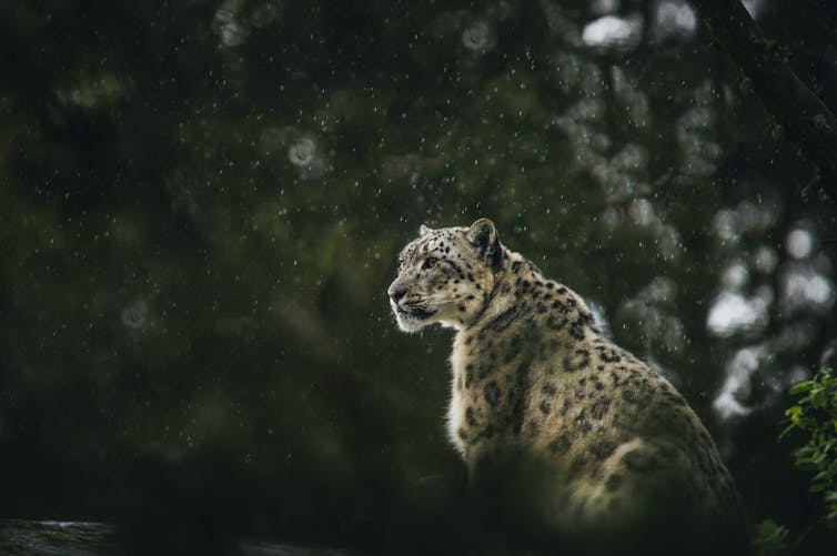
Have you ever watched a nature documentary and marvelled at the intricate dance of life unfolding on screen? From the smallest insect to the largest predator, every creature plays a role in the grand performance of our planet’s biosphere. But what happens when one of these performers disappears?
In this post, we delve into our recent article Estimating co-extinction risks in terrestrial ecosystems just published in Global Change Biology, in which we discuss the cascading effects of species loss and the risks of ‘co-extinction’.
But what does ‘co-extinction’ really mean?
Imagine an ecosystem as a giant web of interconnected species. Each thread represents a relationship between two species — for example, a bird that eats a certain type of insect, or a plant that relies on a specific species of bee for pollination. Now, what happens if one of these species in the pair disappears? The thread breaks and the remaining species loses an interaction. This could potentially lead to its co-extinction, which is essentially the domino effect of multiple species losses in an ecosystem.
A famous example of this effect can be seen with the invasion of the cane toad (Rhinella marina) across mainland Australia, which have caused trophic cascades and species compositional changes in these communities.
The direct extinction of one species, caused by effects such as global warming for example, has the potential to cause other species also to become extinct indirectly.
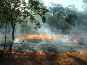
Climate change is one of the main drivers of species loss globally. We know more plants and animals will die as heatwaves, bushfires, droughts and other natural disasters worsen.
But to date, science has vastly underestimated the true toll climate change and habitat destruction will have on biodiversity. That’s because it has largely neglected to consider the extent of “co-extinctions”: when species go extinct because other species on which they depend die out.
Our new research shows 10% of land animals could disappear from particular geographic areas by 2050, and almost 30% by 2100. This is more than double previous predictions. It means children born today who live to their 70s will witness literally thousands of animals disappear in their lifetime, from lizards and frogs to iconic mammals such as elephants and koalas.
But if we manage to dramatically reduce carbon emissions globally, we could save thousands of species from local extinction this century alone.
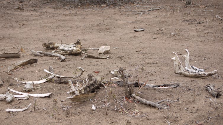
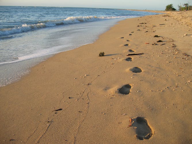
Ravages of drought will only worsen in coming decades. CJA Bradshaw
An extinction crisis unfolding
Every species depends on others in some way. So when a species dies out, the repercussions can ripple through an ecosystem.
For example, consider what happens when a species goes extinct due to a disturbance such as habitat loss. This is known as a “primary” extinction. It can then mean a predator loses its prey, a parasite loses its host or a flowering plant loses its pollinators.
A real-life example of a co-extinction that could occur soon is the potential loss of the critically endangered mountain pygmy possum (Burramys parvus) in Australia. Drought, habitat loss, and other pressures have caused the rapid decline of its primary prey, the bogong moth (Agrotis infusa).
I’m very chuffed today to signal the publication of what I think is one of the most important contributions to the persistent conundrum surrounding the downfall of Australia’s megafauna many tens of millennia ago.
Sure, I’m obviously biased in that assessment because it’s a paper from our lab and I’m a co-author, but if readers had any inkling of the work that went into this paper, I think they might consider adopting my position. In addition, the injection of some actual ecology into the polemic should be viewed as fresh and exciting.
Having waded into the murky waters of the ‘megafauna debate’ for about a decade now, I’ve become a little sensitive to even a whiff of binary polemic surrounding their disappearance in Australia. Acolytes of the climate-change prophet still beat their drums, screaming for the smoking gun of a spear sticking out of a Diprotodon‘s skull before they even entertain the notion that people might have had something to do with it — but we’ll probably never find one given the antiquity of the event (> 40,000 years ago). On the other side are the blitzkriegers who declaim that human hunting single-handedly wiped out the lot.
Well, as it is for nearly all extinctions, it’s actually much more complicated than that. In the case of Sahul’s megafauna disappearances, both drivers likely contributed, but the degree to which both components played a part depends on where and when you look — Fred Saltrédemonstrated that elegantly a few years ago.
So, why does the polemic persist? In my view, it’s because we have largely depended on the crude comparison of relative dates to draw our conclusions. That is, we look to see if some climate-change proxy shifted in any notable way either before or after an inferred extinction date. If a particular study claims evidence that a shift happened before, then it concludes climate change was the sole driver. If a study presents evidence that a shift happened after, then humans did it. Biases in geochronological inference (e.g., spatial, contamination), incorrect application of climate proxies, poor taxonomic resolution, and not accounting for the Signor-Lipps effect all contribute unnecessarily to the debate because small errors or biases can flip relative chronologies on their head and push conclusions toward uncritical binary outcomes. The ‘debate’ has been almost entirely grounded on this simplistically silly notion.
This all means that the actual ecology has been either ignored or merely made up based on whichever pet notion of the day is being proffered. Sure, there are a few good ecological inferences out there from some damn good modellers and ecologists, but these have all been greatly simplified themselves. This is where our new paper finally takes the ecology part of the problem to the next level.
Flinders University Global Ecology postdoc, Dr Farzin Shabani, recently created this astonishing video not only about the results of his models predicting vegetation change in northern Australia as a function of long-term (tens of thousands of years) climate change, but also on the research journey itself!
He provides a brief background to how and why he took up the challenge:
Science would be a lot harder to digest without succinct and meaningful images, graphs, and tables. So, being able to visualise both inputs and outputs of scientific models to cut through the fog of data is an essential element of all science writing and communication. Diagrams help us understand trends and patterns much more quickly than do raw data, and they assist with making comparisons.
During my academic career, I have studied many different topics, including natural hazards (susceptibility & vulnerability risks), GIS-based ensemble modelling, climate-change impacts, environmental modelling at different temporal and spatial scales, species-distribution modelling, and time-series analysis. I use a wide range of graphs, charts, plots, maps and tables to transfer the key messages.
For my latest project, however, I was given the opportunity to make a short animation and visualise my results and the journey itself. I think that my animation inspires asense of wonder, which is among the most important goals of science education. I also think that my animation draws connections to real-life problems (e.g., ecosystem changes as a product of climate change), and also develops an appreciation of the scientific process itself.
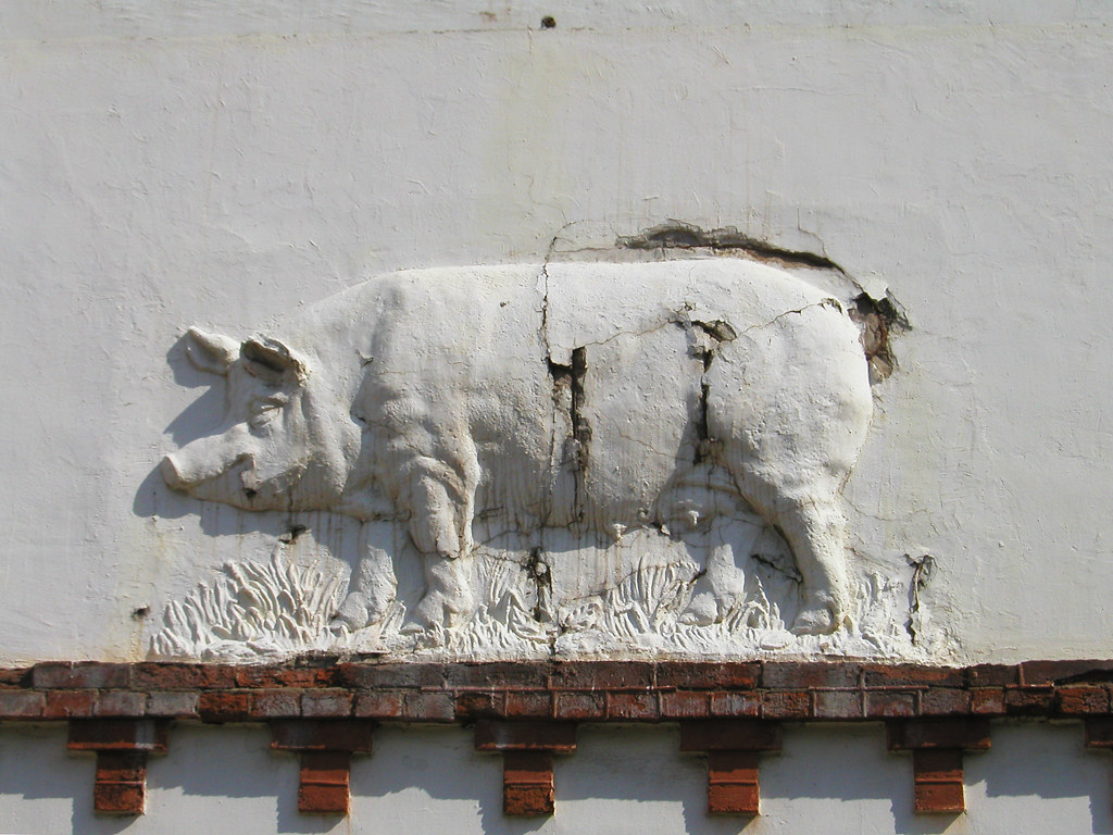
Back in June of this year I wrote (whinged) about the disappointment of writing a lot of ecological models that were rarely used to assist real-world wildlife management. However, I did hint that another model I wrote had assistance one government agency with pig management on Kangaroo Island.
Modelling by the Flinders UniversityGlobal Ecology Laboratory shows the likelihood and feasibility of feral pig eradication under different funding and eradication scenarios. With enough funding, feral pigs could be eradicated from Kangaroo Island in 2 years.
This basically means that because of the model, PIRSA was successful in obtaining enough funding to pretty much ensure that the eradication of feral pigs from Kangaroo Island will be feasible!
Why is this important to get rid of feral pigs? They are a major pest on the Island, causing severe economic and environmental impacts both to farms and native ecosystems. On the agricultural side of things, they prey on newborn lambs, eat crops, and compete with livestock for pasture. Feral pigs damage natural habitats by up-rooting vegetation and fouling waterholes. They can also spread weeds and damage infrastructure, as well as act as hosts of parasites and diseases (e.g., leptospirosis, tuberculosis, foot-and-mouth disease) that pose serious threats to industry, wildlife, and even humans.
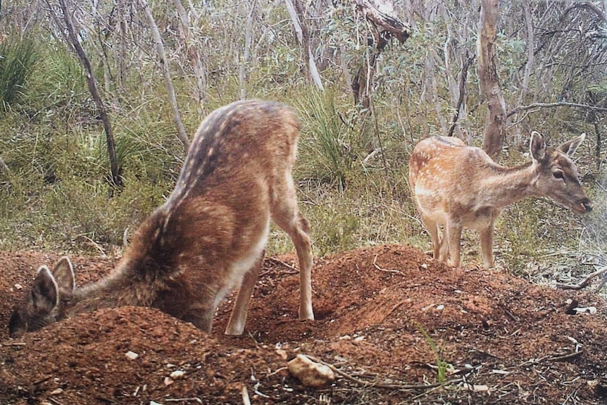
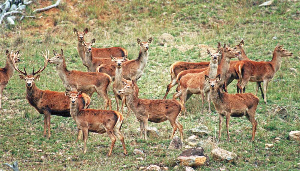
South Australian legislation requires that all landholders cull feral deer on their properties. Despite this, feral deer abundance and distribution are increasing across South Australia. This arises because culling by land managers and government organisations is not keeping pace with rates of population growth, and some landholders are harbouring deer for hunting, whereas some deer escape from deer farms.
There are an estimated 40,000 feral deer in South Australia, and state government agencies are working to ramp up programs to cull feral deer before their numbers reach a point where control is no longer feasible.
Planning such large-scale and costly programs requires that government agencies engage economists to measure the economic impacts of feral deer, and to predict the value of these impacts in the future. That modelling is done regularly by governments, and in the case of pest-control programs, the modelling draws on models of feral deer population growth, farmer surveys about the economic, social, and environmental impacts of feral deer, and analyses of culling programs and trials of new culling techniques.
The economic models predict and compare both the current and future costs of:
deer impacts on pastures, crops, native plants, and social values (including illegal hunting)
culling programs that achieve different objectives (e.g., contain vs. reduce vs. eradicate)
The outputs of the models also inform whether there are sufficient public benefits from the investment of public funds into the culling of feral deer.
This PhD project will collate published and unpublished data to refine models of feral deer distribution and abundance under various culling scenarios. This project will drive both high-impact publications and, because this project builds extensive collaborations with government agencies, the results will inform the management of feral deer in South Australia.
Sure, it’s a tough time for everyone, isn’t it? But it’s a lot worse for the already disadvantaged, and it’s only going to go downhill from here. I suppose that most people who read this blog can certainly think of myriad ways they are, in fact, still privileged and very fortunate (I know that I am).
Nonetheless, quite a few of us I suspect are rather ground down by the onslaught of bad news, some of which I’ve been responsible for perpetuating myself. Add lock downs, dwindling job security, and the prospect of dying tragically due to lung infection, many have become exasperated.
What can we do in addition to shifting our focus to making the future a little less shitty than it could otherwise be? I have a few tips that you might find useful:
As someone who writes a lot of models — many for applied questions in conservation management (e.g., harvest quotas, eradication targets, minimum viable population sizes, etc.), and supervises people writing even more of them, I’ve had many different experiences with their uptake and implementation by management authorities.
Some of those experiences have involved catastrophic failures to influence any management or policy. One particularly painful memory relates to a model we wrote to assist with optimising approaches to eradicate (or at least, reduce the densities of) feral animals in Kakadu National Park. We even wrote the bloody thing in Visual Basic (horrible coding language) so people could run the module in Excel. As far as I’m aware, no one ever used it.
Others have been accepted more readily, such as a shark-harvest model, which (I think, but have no evidence to support) has been used to justify fishing quotas, and one we’ve done recently for the eradication of feral pigs on Kangaroo Island (as yet unpublished) has led directly to increased funding to the agency responsible for the programme.
According to Altmetrics (and the online tool I developed to get paper-level Altmetric information quickly), only 3 of the 16 of what I’d call my most ‘applied modelling’ papers have been cited in policy documents:
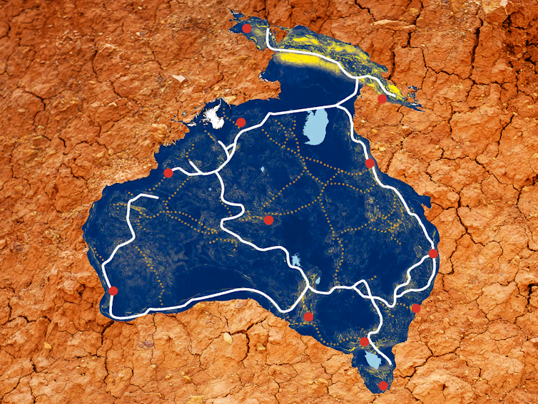
There are many hypotheses about where the Indigenous ancestors first settled in Australia tens of thousands of years ago, but evidence is scarce.
Few archaeological sites date to these early times. Sea levels were much lower and Australia was connected to New Guinea and Tasmania in a land known as Sahul that was 30% bigger than Australia is today.
Our latest research advances our knowledge about the most likely routes those early Australians travelled as they peopled this giant continent.
Modelling human movement requires understanding how people navigate new terrain. Computers facilitate building models, but they are still far from easy. We reasoned we needed four pieces of information: (1) topography; (2) the visibility of tall landscape features; (3) the presence of freshwater; and (4) demographics of the travellers.
We think people navigated in new territories — much as people do today — by focusing on prominent land features protruding above the relative flatness of the Australian continent. Read the rest of this entry »
For many years I’ve been interested in modelling the extinction dynamics of megafauna. Apart from co-authoring a few demographically simplified (or largely demographically free) models about how megafauna species could have gone extinct, I have never really tried to capture the full nuances of long-extinct species within a fully structured demographic framework.
That is, until now.
But how do you get the life-history data of an extinct animal that was never directly measured. Surely, things like survival, reproductive output, longevity and even environmental carrying capacity are impossible to discern, and aren’t these necessary for a stage-structured demographic model?
The answer to the first part of that question “it’s possible”, and to the second, it’s “yes”. The most important bit of information we palaeo modellers need to construct something that’s ecologically plausible for an extinct species is an estimate of body mass. Thankfully, palaeontologists are very good at estimating the mass of the things they dig up (with the associated caveats, of course). From such estimates, we can reconstruct everything from equilibrium densities, maximum rate of population growth, age at first breeding, and longevity.
But it’s more complicated than that, of course. In Australia anyway, we’re largely dealing with marsupials (and some monotremes), and they have a rather different life-history mode than most placentals. We therefore have to ‘correct’ the life-history estimates derived from living placental species. Thankfully, evolutionary biologists and ecologists have ways to do that too.
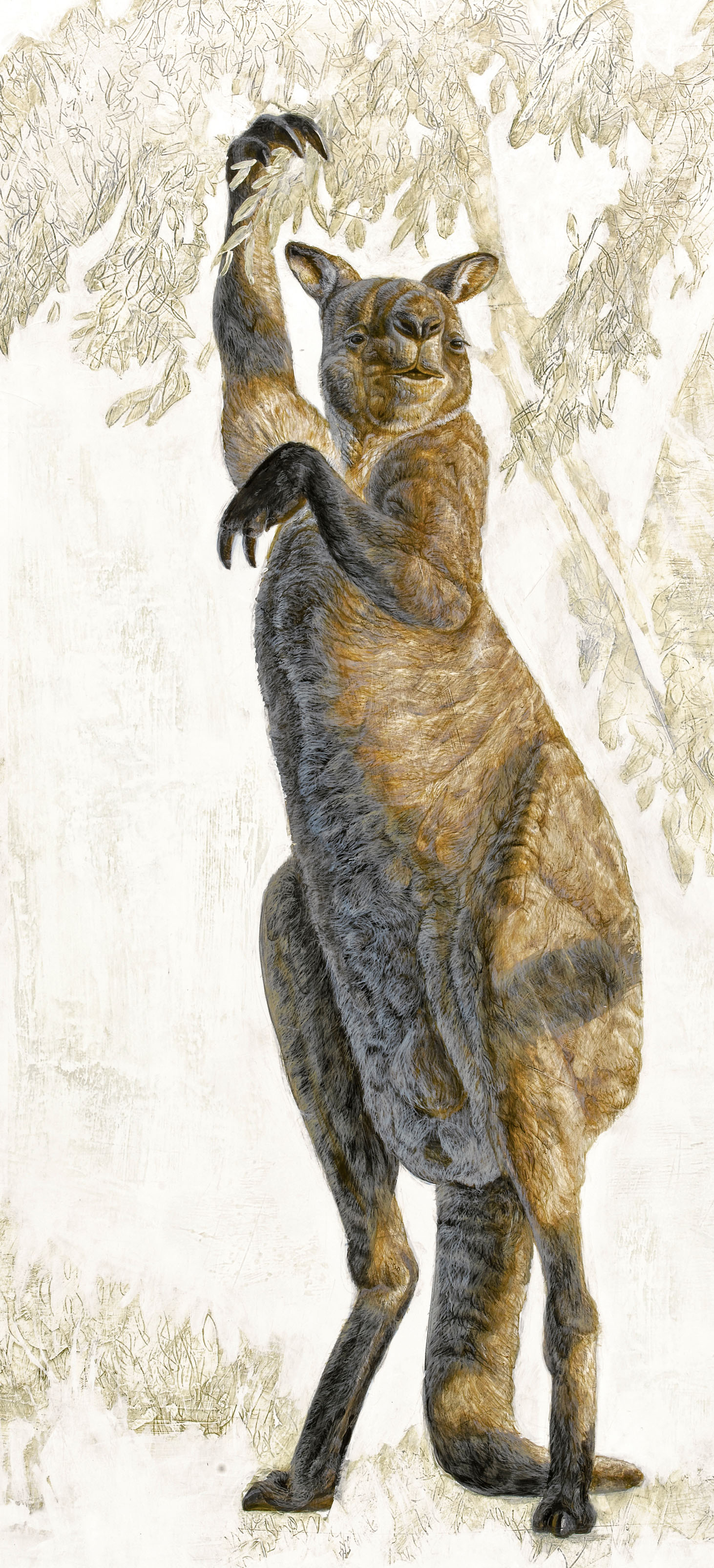
The Pleistocene kangaroo Procoptodon goliah, the largest and most heavily built of the short-faced kangaroos, was the largest and most heavily built kangaroo known. It had an unusually short, flat face and forwardly directed eyes, with a single large toe on each foot (reduced from the more normal count of four). Each forelimb had two long, clawed fingers that would have been used to bring leafy branches within reach.
So with a battery of ecological, demographic, and evolutionary tools, we can now create reasonable stochastic-demographic models for long-gone species, like wombat-like creatures as big as cars, birds more than two metres tall, and lizards more than seven metres long that once roamed the Australian continent.
Ancient clues, in the shape of fossils and archaeological evidence of varying quality scattered across Australia, have formed the basis of several hypotheses about the fate of megafauna that vanished during a peak about 42,000 years ago from the ancient continent of Sahul, comprising mainland Australia, Tasmania, New Guinea and neighbouring islands.
There is a growing consensus that multiple factors were at play, including climate change, the impact of people on the environment, and access to freshwater sources.
Just published in the open-access journal eLife, our latest CABAH paper applies these approaches to assess how susceptible different species were to extinction – and what it means for the survival of species today.
Using various characteristics such as body size, weight, lifespan, survival rate, and fertility, we (Chris Johnson, John Llewelyn, Vera Weisbecker, Giovanni Strona, Frédérik Saltré & me) created population simulation models to predict the likelihood of these species surviving under different types of environmental disturbance.
We compared the results to what we know about the timing of extinction for different megafauna species derived from dated fossil records. We expected to confirm that the most extinction-prone species were the first species to go extinct – but that wasn’t necessarily the case.
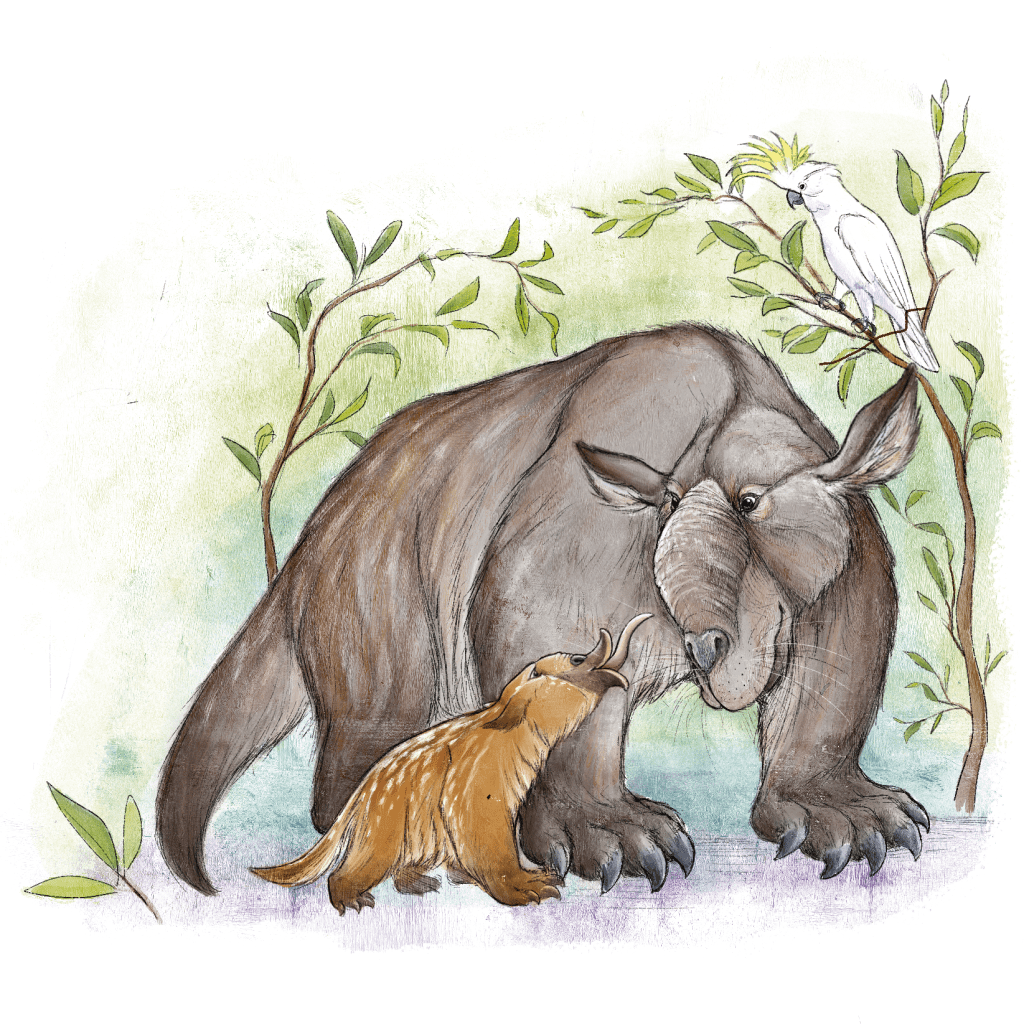
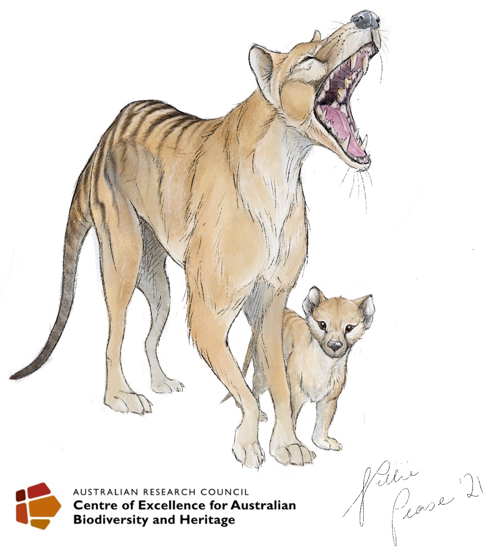
While we did find that slower-growing species with lower fertility, like the rhino-sized wombat relative Diprotodon, were generally more susceptible to extinction than more-fecund species like the marsupial ‘tiger’ thylacine, the relative susceptibility rank across species did not match the timing of their extinctions recorded in the fossil record.
Indeed, we found no clear relationship between a species’ inherent vulnerability to extinction — such as being slower and heavier and/or slower to reproduce — and the timing of its extinction in the fossil record.
In fact, we found that most of the living species used for comparison — such as short-beaked echidnas, emus, brush turkeys, and common wombats — were more susceptible on average than their now-extinct counterparts.
However, this time I’ve strayed from my recent bibliometric musings and developed something that’s more compatible with the core of my main research and interests.
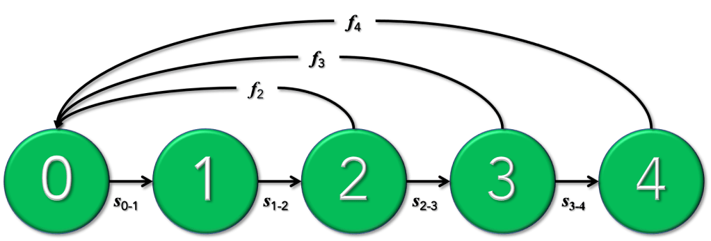
Over the years I’ve taught many students the basics of population modelling, with the cohort-based approaches dominating the curriculum. Of these, the simpler ‘Leslie’ (age-classified) matrix models are both the easiest to understand and for which data can often be obtained without too many dramas.
But unless you’re willing to sit down and learn the code, they can be daunting to the novice.
Sure, there are plenty of software alternatives out there, such as Bob Lacy‘s Vortex (a free individual-based model available for PCs only), Resit Akçakaya & co’s RAMAS Metapop ($; PC only), Stéphane Legendre‘s Unified Life Models (ULM; open-source; all platforms), and Charles Todd‘s Essential (open-source; PC only) to name a few. If you’re already an avid R user and already into population modelling, you might be familiar with the population-modelling packages popdemo, OptiPopd, or sPop. I’m sure there are still other good resources out there of which I’m not aware.
But, even to install the relevant software or invoke particular packages in R takes a bit of time and learning. It’s probably safe to assume that many people find the prospect daunting.
It’s for this reason that I turned my newly acquired R Shiny skills to matrix population models so that even complete coding novices can run their own stochastic population models.
I’m almost slightly embarrassed to say that Shiny was so addictive that I ended up making another app.
This new app takes any list of user-supplied digital object identifiers (doi) and fetches their Altmetric data for you.
Why might you be interested in a paper’s Altmetric data? Citations are only one measure of an article’s impact on the research community, whereas Altmetrics tend to indicate the penetration of the article’s findings to a much broader audience.
Altmetric is probably the leading way to gauge the ‘impact’ (attention) an article has commanded across all online sources, including news articles, tweets, Facebook entries, blogs, Wikipedia mentions and others.
Back in April I blogged about an idea I had to provide a more discipline-, gender-, and career stage-balanced way of ranking researchers using citation data.
Most of you are of course aware of the ubiquitous h-index, and its experience-corrected variant, the m-quotient (h-index ÷ years publishing), but I expect that you haven’t heard of the battery of other citation-based indices on offer that attempt to correct various flaws in the h-index. While many of them are major improvements, almost no one uses them.
Why aren’t they used? Most likely because they aren’t easy to calculate, or require trawling through both open-access and/or subscription-based databases to get the information necessary to calculate them.
Hence, the h-index still rules, despite its many flaws, like under-emphasising a researcher’s entire body of work, gender biases, and weighting towards people who have been at it longer. The h-index is also provided free of charge by Google Scholar, so it’s the easiest metric to default to.
So, how does one correct for at least some of these biases while still being able to calculate an index quickly? I think we have the answer.
Since that blog post back in April, a team of seven scientists and I from eight different science disciplines (archaeology, chemistry, ecology, evolution & development, geology, microbiology, ophthalmology, and palaeontology) refined the technique I reported back then, and have submitted a paper describing how what we call the ‘ε-index’ (epsilon index) performs.
I do a lot of grant assessments for various funding agencies, including two years on the Royal Society of New Zealand’s Marsden Fund Panel (Ecology, Evolution, and Behaviour), and currently as an Australian Research Council College Expert (not to mention assessing a heap of other grant applications).
Sometimes this means I have to read hundreds of proposals made up of even more researchers, all of whom I’m meant to assess for their scientific performance over a short period of time (sometimes only within a few weeks). It’s a hard job, and I doubt very much that there’s a completely fair way to rank a researcher’s ‘performance’ quickly and efficiently.
It’s for this reason that I’ve tried to find ways to rank people in the most objective way possible. This of course does not discount reading a person’s full CV and profile, and certainly taking into consideration career breaks, opportunities, and other extenuating circumstances. But I’ve tended to do a first pass based primarily on citation indices, and then adjust those according to the extenuating circumstances.
But the ‘first pass’ part of the equation has always bothered me. We know that different fields have different rates of citation accumulation, that citations accumulate with age (including the much heralded h-index), and that there are gender (and other) biases in citations that aren’t easily corrected.
I’ve generally relied on the ‘m-index’, which is simply one’s h-index divided by the number of years one has been publishing. While this acts as a sort of age correction, it’s still unsatisfactory, essentially because I’ve noticed that it tends to penalise early career researchers in particular. I’ve tried to account for this by comparing people roughly within the same phase of career, but it’s still a subjective exercise.
I’ve recently been playing with an alternative that I think might be a way forward. Bear with me here, for it takes a bit of explaining. Read the rest of this entry »
Earth is now firmly in the grips of its sixth “mass extinction event”, and it’s mainly our fault. But the modern era is definitely not the first time humans have been implicated in the extinction of a wide range of species.
In fact, starting about 60,000 years ago, many of the world’s largest animals disappeared forever. These “megafauna” were first lost in Sahul, the supercontinent formed by Australia and New Guinea during periods of low sea level.
The main way to investigate this question is to build timelines of major events: when species went extinct, when people arrived, and when the climate changed. This approach relies on using dated fossils from extinct species to estimate when they went extinct, and archaeological evidence to determine when people arrived.
Comparing these timelines allows us to deduce the likely windows of coexistence between megafauna and people.
We can also compare this window of coexistence to long-term models of climate variation, to see whether the extinctions coincided with or shortly followed abrupt climate shifts.
Data drought
One problem with this approach is the scarcity of reliable data due to the extreme rarity of a dead animal being fossilised, and the low probability of archaeological evidence being preserved in Australia’s harsh conditions. Read the rest of this entry »
One of the most ancient peopling events of the great diaspora of anatomically modern humans out of Africa more than 50,000 years ago — human arrival in the great continent of Sahul (New Guinea, mainland Australia & Tasmania joined during periods of low sea level) — remains mysterious. The entry routes taken, whether migration was directed or accidental, and just how many people were needed to ensure population viability are shrouded by the mists of time. This prompted us to build stochastic, age-structured human population-dynamics models incorporating hunter-gatherer demographic rates and palaeoecological reconstructions of environmental carrying capacity to predict the founding population necessary to survive the initial peopling of late-Pleistocene Sahul.
—
As ecological modellers, we are often asked by other scientists to attempt to render the highly complex mechanisms of entire ecosystems tractable for virtual manipulation and hypothesis testing through the inevitable simplification that is ‘a model’. When we work with scientists studying long-since-disappeared ecosystems, the challenges multiply.
Add some multidisciplinary data and concepts into the mix, and the complexity can quickly escalate.
This is how we tackled one of these big questions: just how did the first anatomically modern Homo sapiens make it to the continent and survive?
At that time, Australia was part of the giant continent of Sahul that connected New Guinea, mainland Australia, and Tasmania at times of lower sea level. In fact, throughout most of last ~ 126,000 years (late Pleistocene and much of the Holocene), Sahul was the dominant landmass in the region (see this handy online tool for how the coastline of Sahul changed over this period).
This might seem a little left-of-centre for CB.com subject matter, but hang in there, this does have some pretty important conservation implications.
In our quest to be as transdisciplinary as possible, I’ve team up with a few people outside my discipline to put together a PhD modelling project that could really help us understand how human colonisation shaped not only ancient ecosystems, but also our own ancient cultures.
Thanks largely to the efforts of Dr Frédérik Saltré here in the Global Ecology Laboratory, at Flinders University, and in collaboration with Dr Bastien Llamas (Australian Centre for Ancient DNA), Joshua Birchall (Museu Paraense Emílio Goeldi, Brazil), and Lars Fehren-Schmitz (University of California at Santa Cruz, USA), I think the student could break down a few disciplinary boundaries here and provide real insights into the causes and consequences of human expansion into novel environments.
Interested? See below for more details?
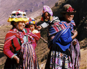
Languages are ‘documents of history’ and historical linguists have developed comparative methods to infer patterns of human prehistory and cultural evolution. The Americas present a more substantive diversity of indigenous language stock than any other continent; however, whether such a diversity arose from initial human migration pathways across the continent is still unknown, because the primary proxy used (i.e., archaeological evidence) to study modern human migration is both too incomplete and biased to inform any regional inference of colonisation trajectories. Read the rest of this entry »
The following is an abridged version of one of the chapters in my recent book, The Effective Scientist, regarding how to prioritise your tasks in academia. For a more complete treatise of the issue, access the full book here.
How the hell do you balance all the requirements of an academic life in science? From actually doing the science, analysing the data, writing papers, reviewing, writing grants, to mentoring students — not to mention trying to have a modicum of a life outside of the lab — you can quickly end up feeling a little daunted. While there is no empirical formula that make you run your academic life efficiently all the time, I can offer a few suggestions that might make your life just a little less chaotic.
Priority 1: Revise articles submitted to high-ranked journals
Barring a family emergency, my top priority is always revising an article that has been sent back to me from a high-ranking journal for revisions. Spend the necessary time to complete the necessary revisions.
Priority 2: Revise articles submitted to lower-ranked journals
I could have lumped this priority with the previous, but I think it is necessary to distinguish the two should you find yourself in the fortunate position of having to do more than one revision at a time.
Priority 3: Experimentation and field work
Most of us need data before we can write papers, so this is high on my personal priority list. If field work is required, then obviously this will be your dominant preoccupation for sometimes extended periods. Many experiments can also be highly time-consuming, while others can be done in stages or run in the background while you complete other tasks.
Priority 4: Databasing
This one could be easily forgotten, but it is a task that can take up a disproportionate amount of your time if do not deliberately fit it into your schedule. Well-organised, abundantly meta-tagged, intuitive, and backed-up databases are essential for effective scientific analysis; good data are useless if you cannot find them or understand to what they refer. Read the rest of this entry »
Just over two years ago I reported the ‘likely’ eradication of feral pigs from Australia’s third-largest (4,405 km2) island — Kangaroo Island. I indicated ‘likely’ because the program still required the proof-of-eradication phase to be completed before an official declaration could be made. Yesterday I had the immense honour to take part in the official…
Have you ever done any research that relied to any degree on Indigenous Knowledges? How did you cite those Knowledges, if at all? It’s probably time we rethink how we engage with Indigenous Knowledge systems. In a new article published in BioScience, we — a large group of Indigenous and non-Indigenous scholars in Australia —…
A recent paper, co-authored with the late Paul Ehrlich, reveals that the global human population has surpassed Earth’s sustainable capacity. It highlights the dire implications for food security, climate stability, and wellbeing. The study underscores that immediate changes in consumption and population management are crucial for a sustainable future.


 I do a lot of grant assessments for various funding agencies, including two years on the Royal Society of New Zealand’s Marsden Fund Panel (
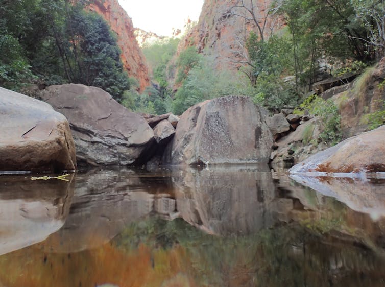
 This might seem a little left-of-centre for